Modeling Run Production June 19, 2010
Posted by tomflesher in Baseball, Economics.Tags: Baseball, economics, regression, run production, sports economics
trackback
A baseball team can be thought of as a factory which uses a single crew to operate two machines. The first machine produces runs while the team bats, and the second machine produces outs while the team is on fields. This is a somewhat abstract way to look at the process of winning games, because ordinarily machines have a fixed input and a fixed output. In a box factory, the input comprises man-hours and corrugated board, and the output is a finished box. Here, the input isn’t as well-defined.
Runs are a function of total bases, certainly, but total bases are functions of things like hits, home runs, and walks. Basically, runs are a function of getting on base and of advancing people who are already on base. Obviously, the best measure of getting on base is On-Base Percentage, and Slugging Average (expected number of bases per at-bat) is a good measure of advancement.
OBP wraps up a lot of things – walks, hits, and hit-by-pitch appearances – and SLG corrects for the greater effects of doubles, triples, and home runs. That doesn’t account for a few other things, though, like stolen bases, sacrifice flies, and sacrifice hits. It also doesn’t reflect batter ability directly, but that’s okay – the stats we have should represent batter ability since the defensive side is trying to prevent run production. The model might look something like this, then:
This is the simplest model we can start with – each factor contributes a discrete number of runs. If we need to (and we probably will), we can add terms to capture concavity of the marginal effect of different stats, or (more likely) an interaction term for SLG and, say, SB, so that a stolen base is worth more on a team where you’re more likely to be brought home by a batter because he’s more likely to give you extra bases. As it is, however, we can test this model with linear regression. The details of it are behind the cut.
I’m using a dataset (available on request) of American League data pulled from Baseball-Reference.com’s Leagues page. I’m using the AL only because I don’t want to correct for the designated hitter’s differential runs.
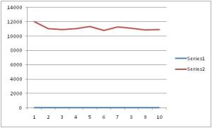
The first thing I need to do is decide whether to add a trend correction.
I don’t have to account for a time trend, so I’m just going to use the team-level data. Using linear regression, I fitted the model above and got the following output:
| Value | Std Err | t-value | p-value | Signif | |
| Intercept | -904.638 | 51.68286 | -17.504 | 0.00000 | 1.00000 |
| OBP | 2893.123 | 233.7059 | 12.379 | 0.00000 | 1.00000 |
| SLG | 1601.076 | 122.3527 | 13.086 | 0.00000 | 1.00000 |
| SB | -0.01907 | 0.06415 | -0.297 | 0.76680 | 0.23320 |
| SF | 0.65975 | 0.25356 | 2.602 | 0.01030 | 0.98970 |
| SH | 0.28282 | 0.17445 | 1.621 | 0.10730 | 0.89270 |
Multiple R-squared: 0.9164, Adjusted R-squared: 0.9132
It looks like OBP and SLG are in fact highly significant, with each sac fly corresponding to about two-thirds of a run scored, a sac bunt corresponding to about .28 runs scored, and a stolen base actually having a negative effect (but it’s only significant at about the 23% level, so we can’t be sure it’s actually different from zero). This model explains about 91% of the variation in run scoring, which is reasonable since it ignores pitching and defense entirely.
This could be tightened up a bit, but as it stands it gives us a reasonable idea of how runs are produced.

Comments»
No comments yet — be the first.