Quality Starts and Differential Luck July 12, 2014
Posted by tomflesher in Baseball, Economics.Tags: quality starts, Zack Wheeler
add a comment
 On July 11, Zack Wheeler gave the Mets a quality start by either definition – he pitched 6 2/3 innings and allowed only one run for a game score of 64. The Mets managed to convert it into a win, which they’ve managed to do in 27 of their 46 wins thus far this year. Zack’s made 12 quality starts this year (by the sabermetric definition of a game score of 50 or more), but the Mets have managed to convert only 5 of them into Ws for Zack; the team is 7-5 in those games, while Zack himself is 5-2. That’s a far cry from the Giants’ freakish Tim Lincecum (9-0 in 12 quality starts) and the Angels’ Garrett Richards (10-0 in 15 quality starts). (The whole list of pitchers with quality starts so far is here.)
That got me thinking – which teams do the best at converting quality starts into wins? Which teams are the worst? What’s the relationship? I grabbed all of these numbers and put them together into a spreadsheet in order to play with them.
First, a quick review of terms: A cheap win is a pitcher win in a non-quality start. A tough loss is a pitcher loss in a quality start. “Luck” is whatever I happen to be measuring at the moment, but today ‘luck differential’ refers to the difference between the percentage of wins that are cheap and the percentage of losses that are tough; in other words, luck differential = 100*[(CW/W) – (TL/L)]. For an individual pitcher, these are fairly random occurrences – no pitcher in MLB today hits reliably enough to consistently earn himself cheap wins – but it seems that aggregating by team allows for the quality of batting to smooth out over a large number of games.
The Texas Rangers lead the league in this sort of luck differential, with 4 of their 38 wins coming cheaply for over 10% cheap wins but only 2 of their 55 losses tough (3.64); the Atlanta Braves have the worst luck differential in the league with a high proportion of tough losses (17/42, or 39.53%) and a low number of cheap wins (3/50, or 6%) for a total of -33.53. The Mets themselves convert less than 50% of their quality starts into wins for the starting pitcher.
These numbers are indicative of a general trend. The more quality starts a team has, the more negative its luck differential is (ρ = -.72 – an extremely strong correlation) and the more wins a team has, the more negative its luck differential is (ρ = -.20 – a bit weaker). Essentially, teams with more quality starts generate more wins (ρ = .56), regardless of the fact that sometimes they lose those quality starts, too. Surprisingly, the Mets have a -21.67 luck differential, one of the most negative in the league, probably due to the fact that they convert so few quality starts into wins.
Wins and Revenue March 31, 2014
Posted by tomflesher in Baseball, Economics.Tags: linear model, Marginal Revenue Product of a win, Revenue, Wins
add a comment
Forbes has released its annual list of baseball team valuations. This is interesting because it accounts for all of the revenue that each team makes, ignoring a lot of the broader factors that play into what causes a team’s value to rise or fall. It also includes a bunch of extra data, including which teams’ values are rising, which are falling, and what each team’s operating income is for the year.
Without getting too in-depth, there are a lot of interesting relationships we can observe by crunching some of the numbers. First, the relationship between wins and revenue is often taken for granted, but the correlation is really very small – only about .26. That means that there’s a great deal more in play determining revenue than just whether a team wins or loses. (This, of course, assumes a linear relationship – one win is worth a fixed dollar amount, and that fixed dollar amount is the same for every team. Correcting this for local income – allowing a win to be worth more in New York than in Pittsburgh – would be an easy extension.)
Under the same assumptions, we can also run a quick linear regression to determine what an average team’s revenue would be at 0 wins and then determine what each marginal win’s revenue product is. Those numbers tell us that, roughly, a 0-win team would make about $129.68 million dollars, gaining around $1.31 million for each win. Again, though, there are a lot of problems with this – obviously, a 0-win team doesn’t exist and would probably have significantly lower revenue than we’d estimate. Even the worst team last year came in at 51 wins. Also, the p-values don’t exactly inspire confidence – the $130 million figure is significant at the 10% level, but the Wins factor comes in around 16%. That’s a pretty chancy number.
Extending it out to include a squared value for wins, we come up with numbers that are astonishingly nonpredictive – the intercept drops to -$34.9 million for a 0-win team (much more reasonable!) with the expected positive marginal value for wins ($5.6 million) and a negative coefficient for squared wins (-$.027), indicating that wins have a decreasing marginal effect as would be predicted. (Once you have 97 wins, the 98th doesn’t usually provide much value.) However, those numbers are basically no better than chance, with respective p-values of .936, .619, and .701. Although the signs look nice, the magnitudes are up in the air.
The sanest model that I can come up with is a log-log regression – that is, starting off with the natural log of revenue and regressing it on the natural log of the number of wins. This gives you an elasticity – a value that explains a percentage change in revenue for a 1% change in the number of wins. This isn’t the most realistic value, of course, since baseball teams play a fixed number of games, but the values look much better – the model looks like:
log(Revenue) = 3.6608 + .4058*log(Wins)
The 3.6608 value is highly significant (p = .00299) and the .4058 coefficient on the number of wins is the strongest we’ve seen yet (p = .1253). It still gives us an unfortunate $38 million operating budget for a zero-win team, but says that doubling a team’s wins should give a 40% increase in revenue. That seems a bit more reasonable.
There are a couple of other, nicer functional forms we could use, but for now, that’s the best we can do with purely linear models.
Spitballing: Position Players Moving Around January 24, 2014
Posted by tomflesher in Baseball, Economics.Tags: Lucas Duda, Spitballing
add a comment
Earlier this week, I posted about Lucas Duda and how he’s being forced out of his natural position. This came up a few years ago for the Mets as well, when Angel Pagan was being forced out of the outfield – many fans suggested pushing him to second base (in the hole now filled by Daniel Murphy). The sense seems to be that players can move freely around the field, going wherever the team needs them. There are a couple of theories on this, and a couple of good examples, but it doesn’t always work out.
Typically, the best moves take someone from a more defensively-demanding position and move him to one that’s less so. Victor Martinez still catches occasionally, but he’s made a move almost entirely to the DH role and played more games at first base last year. Alex Rodriguez has also made some moves in that direction, moving from the very demanding shortstop position to the slightly less difficult third base (perversely, to allow the much lousier Derek Jeter to stay in his position), and mostly toward DH these days. Johnny Damon and Jorge Posada were among the revolving door of older Yankees to do time out of position at first base over the past few years, with varying degrees of success. On the other hand, even moves down the defensive spectrum don’t always work. Gary Sheffield was famously described as “painful to watch” at first by Michael Kaye. Kevin Youkilis was solid in his move from third to first, but the extra speed required for left field left him looking like he couldn’t hack it, and even though the corner positions are great places to stick a team’s best sluggers, it rarely makes sense to move a broken-down catcher there instead of to first or (rarely) third. Even a solid third baseman wouldn’t necessarily have the ability to cover ground needed by an outfielder, even if he had the requisite ability to predict the ball’s flight – a skill that probably needs time in the field to develop.
Pitching is kind of a weird exception. The best example in recent memory has to be Rick Ankiel, whose meltdown on the mound during the World Series led to his second career as an outfielder. On the opposite side, Juan Salas went from being a cannon-armed third baseman to pitching reasonably well, and the Dodgers’ Kenley Jansen has saved 53 games for the Dodgers since being converted from light-hitting catcher to closer. (He also has a lifetime .500/.667/.500 batting line, in the “Utterly Meaningless Statistics” category.) Similarly, Ike Davis went from being his college team’s Friday-night starter to the least defensively-demanding position (first base) in the majors.
Defensive position moves tend to be difficult to make. In Duda’s case, he’d technically be moving up the defensive spectrum, but it’s hard to even consider the speed required to be a competent outfielder on the same scale as the abilities of an infielder. It’s unremarkable to me that Johnny Damon was able to move to first, but putting Youkilis in left field a few years ago was a true head-scratcher. In order to move a player freely between the infield and the outfield, you’ll need a special kind of player unless you’re willing to give up a lot defensively. As an economist, I’m all about specialization given constraints; Duda’s constraints are just too tight to make this move work.
Is Bobby Abreu a good investment for the Phillies? January 23, 2014
Posted by tomflesher in Baseball, Economics.Tags: Bobby Abreu, Jim Thome, Kelly Dugan, Phillies, Tyson Gillies, Zach Collier
add a comment
Bobby Abreu signed with the Phillies on a minor league deal, offering him $800,000 if he makes the major league squad. He’s coming off a solid Winter League season in Venezuela, in which he hit .322/.416/.461. His deal is a bit smaller than the one the Phils offered Jim Thome for 2012, when Thome was 41 (Abreu is 39). Of course, Thome was coming off of a much heavier-slugging season- his OPS in 2011 was .838, almost as high as Abreu’s Venezuelan OPS (and swamping his 2012 Majors OPS of .693). He might play the field on occasion (as Thome did, playing first base in 2012 for the first time since the Bush administration), but the Phils’ corner outfield is pretty solidly set up with Marlon Byrd and Domonic Brown starting.
Thome and Bobby both represent an odd trend – it’s not surprising, really, that the Phillies would want to bring back some of their old sluggers for nostalgia purposes, and they did employ Matt Stairs for longer than they should have – but the trend for a while was toward specialization of pinch hitters into the DH role in the American League. Thome started four games at first base for the Phillies in 2012, but otherwise appeared almost exclusively as a pinch hitter or DH (and in fact was traded to Baltimore once the Phillies’ interleague play ended). Bobby still has more in the tank defensively than Thome did, it seems, but he probably won’t start man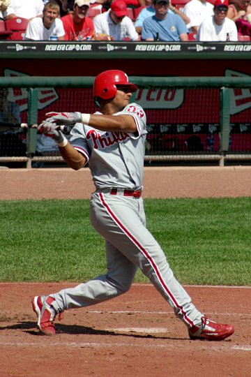 y more games than Thome did.
Given that the Phillies are going to use Abreu the way they used Thome, this doesn’t look like a bad deal. In order to be a reserve outfielder and present some value, Abreu will only have to beat out a few arms in spring training. He’s not in direct competition with John Mayberry, since Mayberry’s a right-handed bat. The Phils have three left-handed minors outfield prospects on their 40-man roster – Zach Collier, Kelly Dugan, and Tyson Gillies. Based on his 2013 numbers, Collier probably isn’t ready – at AA Reading, he hit .222/.310/.348. Dugan, who like Collier was born in September of 1990, looks like he might be better off, but only slightly – his .264/.299/.472 line in 56 AA games (plus slightly better numbers in 56 games at high A) indicate some solid power, but not much plate discipline. Of the three, Gillies (who’s two years older) may be the most mature, but his .264/.312/.477 line doesn’t represent much of a marginal improvement over Dugan. Plus, when he was promoted to AAA Lehigh Valley, he struggled, with a sub-.600 OPS.
From a development perspective, Collier and Dugan might be a better investment, but neither of them is a franchise player, at least based on numbers alone. Abreu represents a nice left-handed insurance bat off the bench.
Ike Davis and his 12% raise January 21, 2014
Posted by tomflesher in Baseball, Economics.Tags: Ike Davis, Mets, Pythagorean expectation
add a comment
So, Ike Davis was pretty lousy last year. He batted .205/.326/.334 in an injury-shortened season with 106 total bases on 377 plate appearances, meaning he expected to make it to first a bit over a quarter of the time. Throw in his paltry home run figures and a handful of doubles, and you’re not looking at a major-league first baseman; his 0.2 wins above replacement put him in the company of Lyle Overbay and Garrett Jones.
Now that that’s out of the way, I’d like to point out that Overbay played 142 games and Jones played 144; Davis definitely presented more bang for your buck than those two, especially since he was earning $3.125 million. He’ll be getting a 12% raise this year, having re-signed for $3.5 million. Again, his numbers were pretty lousy.
But if you add up all of Davis’s appearances as a starter, you’ll see that the Mets scored 354 runs in those games, and allowed 376, meaning that the Pythagorean expectation for those games is 0.46989 – that corresponds to an expectation of about 76 wins over a 162-game season (or 41 wins over Davis’ tenure). The Mets’ overall winning percentage was .457 (74 wins), and their Pythagorean expectation was about .45, corresponding to around 73 wins; but without Davis, the team scored 265 runs and allowed 308, leading to an expectation of .425 and around 69 wins on the season. Additionally, the team actually won only 39 of the 87 games Davis started, for about a .45 winning percentage – right on with their season-long expectation, and two wins below expectation.
Now, there are some caveats. When Davis was active, the team was still doing its best to win, and players like John Buck and Marlon Byrd were still active. Toward the end of the season, the Mets moved more toward development and away from trying to win every game. It’s therefore entirely possible that the effect of having Davis start the game are wrapped up in the team’s changing fortunes. Still, the team would have been expected to perform better with Davis in the lineup, at least according to the Pythagorean expectation formula, and actually underperformed.
Comparing Contracts: Parnell and Gee January 20, 2014
Posted by tomflesher in Baseball, Economics.Tags: Bobby Parnell, comparing contracts, Dillon Gee, Mets
add a comment
A few days ago, Bobby Parnell and Dillon Gee both re-signed with the Mets; though there are some incentives in Parnell’s deal, he’ll be making $3.7 million to Gee’s $3.625 million. Those numbers were oddly close (and the contracts similar despite the difference in position), so I decided to check out the players’ recent statistics. Since the players are each negotiating one-year deals, and these players are neither very old or very young, it seems reasonable to treat the best predictor of future performance as the players’ most recent performance.
Gee started 32 games (almost exactly every fifth game) in 2013 to a 3.62 ERA and a .301 opposing BABIP. The median numbers for starters with 162 or more innings pitched were about 3.51 and .295, so Gee is performing almost exactly like a full-time starter (and thus presumably a bit better than your average pitcher). Gee’s performance corresponds to 2.2 wins above replacement, a shade below the median of 3.0 for full-time starters.
I’m not Parnell’s biggest fan, and his season was shortened by an injury (causing him to miss all of August), so I expected the numbers not to operate in his favor. However, his 2.16 ERA is well below the median of relievers with 40 appearances or more, and his 0.7 WAR is right on the median. Oddly, his BABIP at .268 is much lower than the median of .290, indicating that he’s benefiting, to some degree, from good fielding behind him. If we restrict the numbers to only pitchers with 15 saves or more (all 32 of them), those medians adjust to 2.645, 1.4, and .277, respectively, keeping him on the good side of ERA and BABIP but cutting his WAR performance considerably. Let’s see if we can extrapolate – in 104 team games, Parnell played 49, meaning that he played in about 47% of the team’s games. At that pace, he probably would have been put into about 27 more games, meaning his current stats are about 65% of what his season stats might have been. In that case, let’s hold his BABIP and ERA constant and extend his WAR to 1.08 (by dividing by .65). That would have ranked him with Huston Street and Addison Reed – much better company than his current competition. It also, interestingly, would have put him much closer to Gee’s WAR, at a higher-leverage position.
Again, I’m not Parnell’s biggest fan, and I was skeptical about this deal. Assuming that the injury hasn’t harmed him, though, Parnell’s contract really does make sense compared to Gee’s.
Home Runs Per Game: A bit more in-depth December 23, 2011
Posted by tomflesher in Baseball, Economics.Tags: AR, autoregression, baseball-reference.com, home runs, home runs per plate appearance, linear regression, talent pool dilution
add a comment
I know I’ve done this one before, but in my defense, it was a really bad model.
I made some odd choices in modeling run production in that post. The first big questionable choice was to detrend according to raw time. That might make sense starting with a brand-new league, where we’d expect players to be of low quality and asymptotically approach a true level of production – a quadratic trend would be an acceptable model of dynamics in that case. That’s not a sensible way to model the major leagues, though; even though there’s a case to be made that players being in better physical condition will lead to better production, there’s no theoretical reason to believe that home run production will grow year over year.
So, let’s cut to the chase: I’m trying to capture a few different effects, and so I want to start by running a linear regression of home runs on a couple of controlling factors. Things I want to capture in the model:
- The DH. This should have a positive effect on home runs per game.
- Talent pool dilution. There are competing effects – more batters should mean that the best batters are getting fewer plate appearances, as a percentage of the total, but at the same time, more pitchers should mean that the best pitchers are facing fewer batters as a percentage of the total. I’m including three variables: one for the number of batters and one for the number of pitchers, to capture those effects individually, and one for the number of teams in the league. (All those variables are in natural logarithm form, so the interpretation will be that a 1% change in the number of batters, pitchers, or teams will have an effect on home runs.) The batting effect should be negative (more batters lead to fewer home runs); the pitching effect should be positive (more pitchers mean worse pitchers, leading to more home runs); the team effect could go either way, depending on the relative strengths of the effects.
- Trends in strategy and technology. I can’t theoretically justify a pure time trend, but I also can’t leave out trends entirely. Training has improved. Different training regimens become popular or fade away, and some strategies are much different than in previous years. I’ll use an autoregressive process to model these.
My dependent variable is going to be home runs per plate appearance. I chose HR/PA for two reasons:
- I’m using Baseball Reference’s AL and NL Batting Encyclopedias, which give per-game averages; HR per game/PA per game will wash out the per-game adjustments.
- League HR/PA should show talent pool dilution as noted above – the best hitters get the same plate appearances but their plate appearances will make up a smaller proportion of the total. I’m using the period from 1955 to 2010.
After dividing home runs per game by plate appearances per game, I used R to estimate an autoregressive model of home runs per plate appearance. That measures whether a year with lots of home runs is followed by a year with lots of home runs, whether it’s the reverse, or whether there’s no real connection between two consecutive years. My model took the last three years into account:

Since the model doesn’t fit perfectly, there will be an “error” term, 

The results:

The DH and batter effects aren’t statistically different from zero, surprisingly; the pitching effect and the team effect are both significant at the 95% level. Interestingly, the team effect and the pitching effect have opposite signs, meaning that there’s some factor in increasing the number of teams that doesn’t relate purely to pitching or batting talent pool dilution.
For the record, fitted values of innovations correlate fairly highly with HR/PA: the correlation is about .70, despite a pretty pathetic R-squared of .08.
Bobby Bonilla, Financial Genius? August 1, 2011
Posted by tomflesher in Baseball, Economics.Tags: annuity, Bobby Bonilla, compound interest, deferred compensation, finance, Mets
5 comments
When Bobby Bonilla signed a deferred compensation agreement in 2000, the Mets owed him $5.9 million dollars. Basically, the Mets got to hold on to the $6 million or so (and ended up spending it on payroll), but they had to pay Bonilla back a bit more in interest. His yearly payments are $1,193,248.20, which means that in absolute terms, the Mets are paying him $35,797,446 in total over the next 25 years. Of course, the $1.19 million Bonilla gets today is worth much more than the same-size payment he’ll get in 2036.
Bonilla’s arrangement mimics a financial instrument called an annuity, where a constant payment is made at specific time periods after a specific present sum is invested. The annuity formula is:
![Present Value =Payment \times [\frac{1 - \frac{1}{(1 + r)^t}}{r}]](https://s0.wp.com/latex.php?latex=Present+Value+%3DPayment+%5Ctimes+%5B%5Cfrac%7B1+-+%5Cfrac%7B1%7D%7B%281+%2B+r%29%5Et%7D%7D%7Br%7D%5D&bg=ffffff&fg=666666&s=0&c=20201002)
where r is the annualized interest rate and t is the number of years of payment. Keep in mind, though, that the present value of the annuity isn’t $5.9 million – it’s $5.9 million compounded annually at some rate of interest agreed to by Bonilla and the team for the ten years between the deal and the first payout. In general, that means
![5900000\times(1 + r)^{10} = Payment \times [\frac{1 - \frac{1}{(1 + r)^t}}{r}]](https://s0.wp.com/latex.php?latex=5900000%5Ctimes%281+%2B+r%29%5E%7B10%7D+%3D+Payment+%5Ctimes+%5B%5Cfrac%7B1+-+%5Cfrac%7B1%7D%7B%281+%2B+r%29%5Et%7D%7D%7Br%7D%5D&bg=ffffff&fg=666666&s=0&c=20201002)
Since we know Bonilla’s payout, we can substitute in:
![5900000\times(1 + r)^{10} = 1193248.2 \times [\frac{1 - \frac{1}{(1 + r)^t}}{r}]](https://s0.wp.com/latex.php?latex=5900000%5Ctimes%281+%2B+r%29%5E%7B10%7D+%3D+1193248.2+%5Ctimes+%5B%5Cfrac%7B1+-+%5Cfrac%7B1%7D%7B%281+%2B+r%29%5Et%7D%7D%7Br%7D%5D&bg=ffffff&fg=666666&s=0&c=20201002)
and that solves out neatly to the 8% that the team and Bonilla agreed to. The math checks out so far.
At the time the deal was made, the 8% was 50 basis points (0.5%) below the Prime Rate, the reference rate used by banks in making loans. The average prime rate over the previous year was about 8.16%, and rates had hovered within 75 basis points since September of 1994*, so while interest rates are expected to move, it was very likely that rates would stay similar, at least in the short term. For the record, a 30-year fixed rate mortgage would have cost between 8.15% and 8.25%, so taking into account the long maturity of the loan, it wasn’t a bad deal.
Let’s look at how good a prediction it was. Annualizing prime rates, the Mets could have earned a (full prime) rate of return as follows:

So, the actual value of the $5.9 million on January 1, 2011, was $10,891,903.26, but the agreement pegged the value at

for a difference of about $1.85 million. Bobby’s already better off because historical interest rates didn’t keep up with 8%.
My biggest question is why the Mets agreed to an 8% interest rate then and there to be in effect for the next 35 years. Since I’m not a finance professional, I don’t know whether that’s an industry standard agreement or not, but it seems like the risk of setting an interest rate that far in the future would be far too high. What if the Mets had agreed to the 8% interest rate for ten years and then offered Bonilla a menu of financially equivalent options? All of them would rely on the payment formula:

where t is the number of periods and r is the newly figured interest rate.
One option would be to take the $12,737,657.48 as a lump sum, although that wouldn’t necessarily be a good idea for the Mets. (We know they’re cash strapped.)
The current prime rate is 3.25%, so if we took the lump sum $12,737,657.48 from the original agreement and reamortized it today at 2.75%, Bobby could receive a payment of $711,270.46 over the next 25 years. Similarly, at 2.75%, $1,047,789.14 per year for 15 years or $2,761,502.75 for five years would be equivalent options. Each has a different total cash outlay, but the discount rate means that each of them is worth the same $12,737,657.48 in 2011 dollars.
Bringing it all back, that’s why it’s a little silly to talk about the Mets paying $30 million to defer $6 million in compensation. It’s true that they’ll end up putting more dollars into Bonilla’s hands, but that simply represents Bonilla’s forebearing on the ability to invest that money at current interest rates. It doesn’t matter when you pay him – the money is worth the same amount, and that’s all that matters.
* Historical prime rates here, thanks to the St. Louis Fed and Federal Reserve Economic Data
Mets Fans, Meet Your New Closer July 17, 2011
Posted by tomflesher in Baseball, Economics.Tags: Bobby Parnell, closers, Francisco Rodriguez, Jason Isringhausen, Mets, Pedro Beato
add a comment
It’s been a while since the Mets traded Francisco Rodriguez, the 1982 model, to the Milwaukee Brewers. Mets manager Terry Collins has indicated that Rule 5 draft pick Pedro Beato, cranky old man Jason Isringhausen, and veteran Met Bobby Parnell are in competition for the closer role. Rodriguez had a reputation for being unpredictable, and watching him certainly gave that impression – he pitched wildly and emotionally.
I decided to dig out K-Rod’s stats for this year and figure out what his numbers looked like, using a couple of measures of control: his K/BB ratio (aka ‘control ratio’), his K/9 and BB/9, and then his batters faced per out (BFPO). If Rodriguez is unpredictable, then he should have a relatively high standard deviation for BFPO. With that in mind, if predictability is an important factor in selecting a closer, these stats are relevant for Beato, Isringhausen, and Parnell as well. Here they are, for 2011:
The best number overall is bolded. The best from among the three closer candidates is italicized.

Rodriguez had the best KBB and BB9, as well as the lowest standard deviation, but his BFPO was the highest in the group. Since he wasn’t walking many batters, that indicates that he was giving up a lot of hits or otherwise allowing lots of runners. That’s not good – it breeds high-pressure situations, some of which are bound to result in runs.
Beato had the lowest BFPO, but Parnell led all the other categories for current Mets as well as having a better K/9 than Rodriguez as well. Parnell’s BFPO was only .02 below Frankie’s, and was .15 higher than Beato’s (and about .05 greater than Izzy’s). Without a lot more data, it’s hard to compare these numbers meaningfully. However, over the course of 70 innings, that .15 differential adds up to 31.5 extra baserunners for Parnell above Beato. Parnell’s lower standard deviation means that those runners are going to be spread a bit more evenly than Beato’s, but it’s tough to distinguish the best choice. Isringhausen has been strong as a setup man, and Beato, as a rookie, is still unpredictable.
Parnell will probably come out of this with the closer’s job, but Collins would be a fool not to leave Isringhausen where he is.
Home Field Advantage Again July 12, 2011
Posted by tomflesher in Baseball, Economics.Tags: attendance effects, Baseball, Giants, home field advantage, linear regression, probability, probit, statistics
add a comment
In an earlier post, I discussed the San Francisco Giants’ vaunted home field advantage and came to the conclusion that, while a home field advantage exists, it’s not related to the Giants scoring more runs at home than on the road. That was done with about 90 games’ worth of data. In order to come up with a more robust measure of home field advantage, I grabbed game-by-game data for the national league from the first half of the 2011 season and crunched some numbers.
I have two questions:
- Is there a statistically significant increase in winning probability while playing at home?
- Is that effect statistically distinct from any effect due to attendance?
- If it exists, does that effect differ from team to team? (I’ll attack this in a future post.)
Methodology: Using data with, among other things, per-game run totals, win-loss data, and attendance, I’ll run three regressions. The first will be a linear probability model of the form

where 

As such, I’ll also run a Probit model of the same equation to avoid problems caused by the simplicity of the linear probability model.
Finally, just as a sanity check, I’ll run the same regression, but for runs, instead of win probability. Since runs aren’t binary, I’ll use ordinary least squares, and also control for the possibility that games played in American League parks lead to higher run totals by controlling for the designated hitter:

Since runs are a factor in winning, I have the same expectations about the signs of the beta values as above.
Results:
Regression 1 (Linear Probability Model):

So, my prediction about the attendance betas was incorrect, but only because I failed to account for the squared terms. The effect from home attendance increases as we approach full attendance; the effect from road attendance decreases at about the same rate. There’s still a net positive effect.
Regression 2 (Probit Model):

Note that in both cases, there’s a statistically significant 
Finally, the regression on runs:
Regression 3 (Predicted Runs):
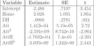
Again, with runs, there is a statistically significant effect from being at home, and a variety of possible attendance effects. For low attendance values, the Home effect is probably swamped by the negative attendance effect, but for high attendance games, the Home effect probably outweighs the attendance effect or the attendance effect becomes positive.
Again, the Home effect is statistically significant no matter which model we use, so at least in the National League, there is a noticeable home field advantage.
