NHL Pythagorean Luck through December 10, 2015 December 11, 2015
Posted by tomflesher in Hockey, Sports.Tags: hockey, NHL, Pythagorean expectation, wins above expectation
add a comment
Below is a plot of NHL teams’ Pythagorean luck through games played on December 10. The bubbles are scaled to the number of wins each team has.

Shockingly, the 12-16 Calgary Flames are 2.4 wins above their expectation, meaning that they should really be a 10-18 or 9-19 team right now. Meanwhile, the Canucks are suffering at 3.4 wins below expectation; at 11-19, they could easily be a .500 team if a few pucks had bounced differently.
Lucky wins for each team follow:
| Team | Lucky Wins |
| Dallas Stars | 2.97 |
| Montreal Canadiens | -1.23 |
| Washington Capitals | 1.58 |
| New York Rangers | -1.24 |
| Los Angeles Kings | 1.38 |
| New York Islanders | -0.77 |
| Detroit Red Wings | 1.09 |
| St. Louis Blues | 1.08 |
| Nashville Predators | 0.30 |
| Ottawa Senators | -0.21 |
| Chicago Blackhawks | -0.29 |
| Boston Bruins | -0.60 |
| Minnesota Wild | -0.23 |
| Florida Panthers | -0.93 |
| Pittsburgh Penguins | 1.28 |
| New Jersey Devils | -0.66 |
| Tampa Bay Lightning | -1.65 |
| Philadelphia Flyers | 1.41 |
| Winnipeg Jets | 0.58 |
| Vancouver Canucks | -3.40 |
| San Jose Sharks | 0.39 |
| Anaheim Ducks | 0.13 |
| Arizona Coyotes | 1.50 |
| Edmonton Oilers | -0.19 |
| Calgary Flames | 2.40 |
| Buffalo Sabres | -1.26 |
| Toronto Maple Leafs | -1.58 |
| Colorado Avalanche | -1.38 |
| Carolina Hurricanes | 0.23 |
| Columbus Blue Jackets | -0.70 |
| League Average | 0.00 |
Evaluating Hockey Analytics (and bonus luck numbers through November 15, 2015) November 16, 2015
Posted by tomflesher in Economics, Hockey, Sports.Tags: Corsi, Fenwick, Hockey analytics, NHL, Pythagorean expectation, Pythagorean luck, Sabres
add a comment
The Buffalo Sabres have been having a weird season. They’ve been outshot and won, they’ve outshot their opponents and lost, and (aside
from starting goalie Chad Johnson) their ice time leader, defenseman Rasmus Ristolainen, is bringing up the rear in relative Corsi and Fenwick stats. Ristolainen has a nasty -9.5 Corsi Rel, while fellow defenders Jake McCabe, Mark Pysyk, and Mike Weber have 8.5, 9.1, and 13.5, respectively. Ristolainen is averaging over 24 minutes a game, with the other three down by six to eight minutes each. What’s more, Ristolainen appears to be pulling his weight – he’s made 45 shots, second only to center Jack Eichel, and has 4 goals with an 8.9 shooting percentage. Ristolainen has 11 points (second only to Ryan O’Reilly with 14) but is tied with Tyler Ennis for the team’s worst +/- at -6. See? Weird year so far.
A lot of that is small sample size, of course. The Sabres are only 17 games into the 82-game season. They are, however, looking awfully lucky so far. Just how lucky? Let’s find out using the same Pythagorean metric that shows up in baseball.
Since Corsi and Fenwick both measure attempts to shoot, they’re noisier than goals. I was curious how much noisier, so I fired up R using the 2014 data and decided to update my post from earlier this year about the optimal Pythagorean exponent for the NHL. In it, I set up three minimization problems, all of them estimating winning percentage (and counting overtime losses as losses – the exponent changes only slightly if you estimate points-percentage instead of wins). Those three problems each minimized the sum of squares, using the Pythagorean formulas. The first used the traditional method of estimating goals and goals against; the second used Corsi For and Corsi Against; the third used Fenwick For and Fenwick Against.
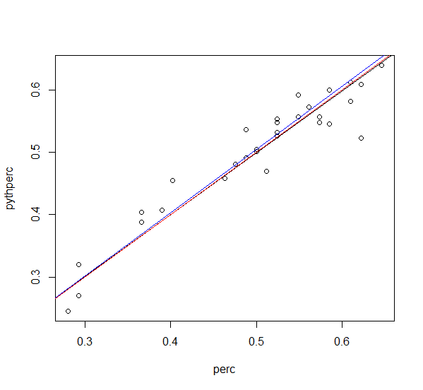
Pythagorean 2.11 in black, Corsi 1.445 in blue, and Fenwick 1.88 in red.
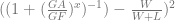
The Goals For/Goals Against form (

The Corsi For/Corsi Against form returns an optimal x of 1.445, but the residual sum of squares ballooned to .24. That means on average the squared error is almost ten times as great – you get a pretty good predictor, but with much more “noise.”
Right in the middle, the Fenwick form yields an optimal x of 1.877, with a residual squared error of .203. It’s a better predictor of wins and losses than the Corsi version, but it’s still not as good a predictor of wins as the simple Goals For/Goals Against form.
Above, I’ve graphed each team’s winning percentage against the Pythagorean (Goals For/Goals Against form), as well as all three trendlines: note that the black Goals line and the red Fenwick line are extremely close, while the blue Corsi line is a bit higher up. Two conclusions can be drawn:
- The Fenwick line is a better predictor than the Corsi line, but the Corsi line appears to bias expected percentage upward. That is, it overestimates the imact of each shot more than goals and Fenwick do.
- Since the Fenwick line is a better predictor, that indicates that Corsi’s inclusion of blocked shots probably does just add noise. Blocked shots are, at least according to this model, of limited predictive value.
Through November 15, Corsi For % had a correlation of .11 with points and .125 with winning percentage; Fenwick For % had correlations of .17 and .19, respectively. Blocked shots had negative correlations in both cases.
Pythagorean luck is defined as the number of wins above expectation. Behind the jump are the numbers, through November 15, demonstrating which teams are lucky and which aren’t.
A Pythagorean Exponent for the NHL March 17, 2015
Posted by tomflesher in Sports.Tags: hockey, luck, NHL, parameter identification, Pythagorean expectation, Sabres
4 comments
A Pythagorean expectation is a statistic used to measure how many wins a team should expect, based on how many points they score and how many they allow. The name ‘Pythagorean’ comes from the Pythagorean theorem, which measures the distance between the two short sides of a right triangle (the hypotenuse); the name reflects the fact that early baseball-centric versions assumed that Runs^2/(Runs^2 + Runs Allowed^2) should equal the winning percentage, borrowing the exponent of 2 from the familiar Pythagorean theorem (a^2 +b^2 =c^2).
The optimal exponent turned out not to be 2 in just about any sport; in baseball, for example, the optimal exponent is around 1.82. This is found by setting up a function – in the case of the National Hockey League, that formula would be 

Porting that exponent into the current season, there are a few surprises. First of all, the Anaheim Ducks have been lucky – almost six full wins worth of luck. It would hardly be surprising for them to tank the last few games of the season. Similarly, the Washington Capitals are on the precipice of the playoff race, but they’re over four games below their expected wins. With 11 games to go, there’s a good chance they can overtake the New York Islanders (who are 3.4 wins above expectation), and they’re likely to at least maintain their wild card status.
On the other end, somehow, the Buffalo Sabres are obscenely lucky. The worst team in the NHL today is actually 4 games better than its expectation. Full luck standings as of the end of March 16th are behind the cut.
Ike Davis and his 12% raise January 21, 2014
Posted by tomflesher in Baseball, Economics.Tags: Ike Davis, Mets, Pythagorean expectation
add a comment
So, Ike Davis was pretty lousy last year. He batted .205/.326/.334 in an injury-shortened season with 106 total bases on 377 plate appearances, meaning he expected to make it to first a bit over a quarter of the time. Throw in his paltry home run figures and a handful of doubles, and you’re not looking at a major-league first baseman; his 0.2 wins above replacement put him in the company of Lyle Overbay and Garrett Jones.
Now that that’s out of the way, I’d like to point out that Overbay played 142 games and Jones played 144; Davis definitely presented more bang for your buck than those two, especially since he was earning $3.125 million. He’ll be getting a 12% raise this year, having re-signed for $3.5 million. Again, his numbers were pretty lousy.
But if you add up all of Davis’s appearances as a starter, you’ll see that the Mets scored 354 runs in those games, and allowed 376, meaning that the Pythagorean expectation for those games is 0.46989 – that corresponds to an expectation of about 76 wins over a 162-game season (or 41 wins over Davis’ tenure). The Mets’ overall winning percentage was .457 (74 wins), and their Pythagorean expectation was about .45, corresponding to around 73 wins; but without Davis, the team scored 265 runs and allowed 308, leading to an expectation of .425 and around 69 wins on the season. Additionally, the team actually won only 39 of the 87 games Davis started, for about a .45 winning percentage – right on with their season-long expectation, and two wins below expectation.
Now, there are some caveats. When Davis was active, the team was still doing its best to win, and players like John Buck and Marlon Byrd were still active. Toward the end of the season, the Mets moved more toward development and away from trying to win every game. It’s therefore entirely possible that the effect of having Davis start the game are wrapped up in the team’s changing fortunes. Still, the team would have been expected to perform better with Davis in the lineup, at least according to the Pythagorean expectation formula, and actually underperformed.
Is ‘luck’ persistent? May 25, 2011
Posted by tomflesher in Baseball, Economics.Tags: American League, Baseball, Pythagorean expectation, wins above expectation
2 comments
I’ve been listening to Scott Patterson’s The Quants in my spare time recently. One of the recurring jokes is Wall Street traders’ use of the word ‘Alpha’ (which usually represents abnormal returns in finance) to refer to a general quality of being skillful or having talent. That led me to think about an old concept I haven’t played with in a while – wins above expectation.
As a quick review, wins above expectation relate a team’s actual wins to its Pythagorean expectation. If the team wins more than expected, it has a positive WAE number, and if it loses more than expected, it has wins below expectation, or, equivalently, a negative WAE. It’s tempting to think of WAE as representing a sort of ‘alpha’ in the traders’ sense – since the Pythagorean Expectation involves groups of runs scored and runs allowed, it generates a probability that a team with a history represented by its runs scored/runs allowed stats will win a given game. If a team has a lot more wins than expected, it seems like that represents efficiency – scoring runs at crucial times, not wasting them on blowing out opponents – or especially skillful management. Alternatively, it could just be luck. Is there any way to test which it is?
It’s difficult. However, let’s break down what the efficiency factor would imply. In general, it would represent some combination of individual player skill (such as the alleged clutch hitting ability) and team chemistry, whether that boils down to on- or off-field factors. Assuming rosters don’t change much over the course of the year, then, efficiency also shouldn’t change much over the course of the year. Similarly, if a manager’s skill was the primary determinant of wins above expectation, then for teams that don’t change managers midyear, we wouldn’t expect much of a change throughout the course of the season. Most managers work up through the minors, so there probably isn’t a major on-the-job training effect to consider.
On the other hand, if wins above expectation are just luck, then we wouldn’t need to place any restrictions on them. Maybe they’d change. Maybe they wouldn’t. Who knows?
In order to test that idea, I pulled some data for the American League off Baseball Reference from last season. I split the season into pre- and post-All-Star Break sets and calculated the Pythagorean expectation (using the 1.81 exponent referred to in Wikipedia) for each team. I found WAE for each team in each session, then found each team’s ‘Alpha’ for that session by dividing WAE by the number of games played. Basically, I assumed that WAE represented extra win probability in some fashion and assumed it existed in every game at about the same level. The results:

As is evident from the table, a whopping 10 out of the 14 teams see a change in the sign of Alpha from before the All-Star Game to after the All-Star Game. The correlation coefficient of Alpha from pre- to post-All-Star is -.549, which is a pretty noisy correlation. (Note also that this very closely describes regression to the mean.) It’s not 0, but it’s also negative, implying one of two things: Either teams become less efficient and/or more badly managed, on average, after the break, or Alpha represents very little more than a realization of a random process, which might just as well be described as luck.
Addendum on Pythagorean Expectation May 20, 2010
Posted by tomflesher in Baseball, Economics.Tags: Baseball, economics, Pythagorean expectation, statistics
1 comment so far
I noted below that the sample size of 13 games is too small to make a determination as to whether the proportions of conditions expected to predict the winning team – the home team, the team with the higher Pythagorean expectation, the team with more runs scored, and the team with the higher run differential – is significantly different from chance. If chance were the only determinant of the winner, then we would expect each proportion to be .5, since you’d expect a randomly-selected home team to win half the games, a randomly-selected team with higher run differential to win half the games, and so on.
Making the standard statistical assumptions, the margin of error using proportions is 


For the simple measure of more runs, the proportion was .31, meaning that the margin of error is 

How Useful is the Pythagorean Expectation? May 18, 2010
Posted by tomflesher in Baseball.Tags: baseball-reference.com, one-game playoffs, Pythagorean expectation, wins above expectation
add a comment
The Pythagorean expectation is a method used to approximate how many wins a baseball team “should” have based on its offense (runs scored) and its defense (runs allowed). As the linked article points out, there are some problems with the formula. As far as I’m concerned, the most useful application of an expected win percentage is to compare teams that are otherwise similar. Let’s say, for example, that I have two teams that have identical records and I want to predict which team will win an upcoming series. In that case, an expected win percentage would be useful to indicate which team has more firepower over time.
What’s the perfect way to test this? One-game playoffs. Behind the cut, I have the results of some number-crunching I did to test whether the Pythagorean expectation generates useful results.
